NuLife Further Analyses
When visualizing the system one can think of a stack of nineteen two-state layers. Eighteen of these layers stand in for the rules, with each layer representing a test (density). The nineteenth layer holds the state for the outer-totalistic automata. Thought of in these terms, system could be seen as a uniform cellular automata with 219 states and a very large and complicated state machine, however, it doesn't seem particularly useful to do so. It is more interesting to look at how the layers work independently and how they affect one another.
Operationally, the test layers treat the nineteenth layer as a mask. Any cells that are “off” in the mask are treated as “off” in the layer. A cell will then decide to be “on” either if all cells and their matching masks are “on”, or if the cell is “off” and at least one of its neighbours is “on”.
The first eighteen layers can be calculated in parallel. The nineteenth layer gets calculated subsequently. This creates a two phase system, with feedback between the phases.
It is possible to consider the behaviour of the layers more-or-less independently, and this is helpful when exploring the underlying mechanics of the system. We can treat a layer and mask combination as a three state cellular automata. Here, 0 means a cell is “off”; 1 means that it is “on”, but not executing the test in question; and, 2 means that the cell is executing the test. However, as we are only modifying the activation of the test and not the mask, the output state of this system can only be 0 or 2. We can examine a single cell and its neighbourhood. For descriptive purposes the neighbourhood can be reduced to only 2 cells, and symmetrical inputs can be ignored. The set of inputs and outputs thus becomes:
000-> 0   001 -> 0   002 -> 2   010 -> 0   020 -> 2
021-> 0   022 -> 2   101 -> 0   102 -> 2   111 -> 0
112-> 0   121 -> 0   122 -> 0   202 -> 2   212 -> 0
222-> 2
Looked at this way, the layer mask combination works like a reaction-diffusion system: An active test will diffuse into an empty cell under any circumstances. However, activation will be inhibited if it comes into direct contact with a different active test layer, as it will either not spread into an already active cell, or it will become inactive.
The behaviour of each of the different layers is identical. Therefore, the inhibition of one layer will lead to reciprocal inhibition of a neighbour cell in another layer. Likewise, diffusion into a cell in one layer allows for diffusion into the same cell from other layers. If we temporarily ignore the second phase of the system, where we determine mask activation, and assume for the moment that any layer being active implies activation of the mask, we can look at a simplified system of interaction between multiple layers. Assuming two layers, and the 1d case, here are some examples of behaviour (time proceeds to the right):
1: 200001  220011  222111  220011  ...
2: 100002  110022  111222  110022  ...

1: 20001  22011  22211  22011  ...
2: 10002  11022  11222  11022  ...

1: 202120202120  220002220002  222022222022  222222222222  222222222222 222222222222 222222222222  ...
2: 201210201210  220002220001  222022222011  222222222211  222222222111 222222221111 222222211111  ...

1: 212020212020  000222000222  002222202222  022222222222  222222222222
2: 121020121020  000222000222  002222202222  022222222222  222222222222

1: 200020102000  220221112200  222200100220  222221112222  222200100222 222221112222  222200100222 ...
2: 200010201000  220112221100  222100200110  221112221111  211100200111 111112221111  111100200111 ...

1: 201020002000  221222022200  201022222220  221222222222  201022222222 221222222222  201022222222 ...
2: 102010002000  122211022200  102011222220  122211122222  102011112222 122211111222  102011111122 ...

1: 222222222002  222222222222  222222222222 ...
2: 222222222001  222222222212  222222222111 ...

1: 222200002222  222220022222  222222222222  222222222222 ...
2: 222200001111  222220011111  222222111111  222221111111 ...
We can see that this simplified system acts to partition space into regions. When one active layer meets another, a narrow membrane is formed that acts to keep the regions separated. In situations where there is a mixed set of active layers in the starting conditions, neighbouring cells will tend to annihilate one another, leaving active cells which can spread. This can lead to the most active layer dominating and suppressing the less active one. Under some conditions, both layers will become active. The system also consistently converges to a largely stable configuration: stable regions of a single active layer, with thin borders that oscillate “off” and “on”. Increasing the number of layers and moving to two dimensions yields roughly analogous results.
In the two dimensional case, starting from random initial conditions, the system forms connected regions of activation, similar to Turing patterns (figure 1). Varying the relative activation of layers in the initial conditions affects how prevalent the layers become, with more active layers becoming more prevalent. Sparseness of activation also has an effect as dense regions with multiple activations will tend to annihilate themselves, leading those regions to become empty, which in turn will allow them to fill with single layers. In an extremely sparse 2D system, activation will spread until layers come into contact with each other, at which point regions will stop spreading in the direction of contact, leading to clean 45 and 90 degree edges.
It is not impossible for the regions formed to have more than one active layer, however, this is uncommon, especially when the number of layers is low. When multiple layers are active in a region, an adjacent region with a sub-set of those layers active will be able to spread into that region and take it over. This can only be prevented if a mutually exclusive region lies between them.
So far in our discussion, a cell's mask is assumed to be active if any of its layers is active. In the full system, the mask activation is dependent on the current mask activation, the active layers and the number of active neighbours. Before looking at the full system, though, we'll first look at what happens if the mask activation is made to be probabilistic, as this will help with an understanding of the system's mechanics.
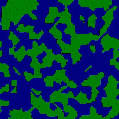
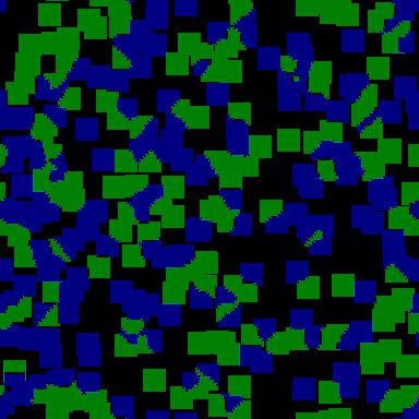
Figure 1. Two layer simplified system in 2D. Left image shows evolution after a few steps. Right is final state. Solid regions forming based on initial prevalence of activation.
There are several ways that stochastic behaviour can be incorporated. The approach taken here is to sum up the number of active layers in a cell and use this as the numerator to a threshold, which is then used to determine if the mask should be active. The comparison is set so that having more active layers will increase the likelihood of activation. By scaling the sum, it is possible to control the minimum amount of activation needed to assure that the mask becomes active. The equation become r < s/t, where r is a random number in the range [0,1), s is the sum of active layers, and t is the threshold scaling. It is possible to run simulations where the threshold starts low and is increased over time.
If the threshold is set sufficiently low (< 1), this system will behave as it did previously (one layer of activation will assure activation of the mask).
Looking at a system with two layers, in addition to the mask, and raising the threshold very slightly (say to 1.1) creates more-or-less the same behaviour, except that inside the uniform regions, there will be occasionally inactive cells. The larger scale patterns formed remain more-or-less static. (Figure 2.)
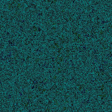
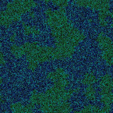
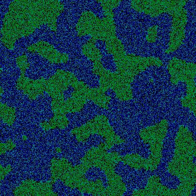
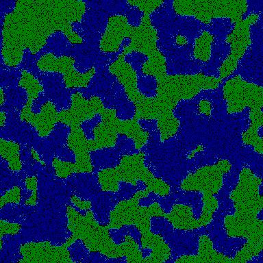
Figure 2. Time evolution of two layer system as threshold is raised. Initially, we see more inactive cells, but cells with more than one active layer start to dominate.
With our two layer system and a threshold of 1.25 to 1.75 we start to see cells which are active in both layers interspersed with the other cells. We also start to see some erosion of regions, and coincident growth of others. As the threshold is increased, the regions become more saturated with two layer activation, and the borders between regions also become broader and clearly saturated with two layer activation. As the threshold is set higher, the active cells become increasingly likely to be active in two layers, and the number of inactive cells begins to increase. With a threshold of 4.0 the cells tend to be either active in both layers or inactive, and at a sufficiently high threshold, the majority of cells will tend to become inactive, until there are no more active cells.
If we add another layer, then the behaviour becomes more interesting. (Figure 3.) Up to a threshold of around 2.25 the system behaves similarly to the two layer system, first with an increase in inactive cells within regions, and then an with an “invasion” of cells with all layers active into the regions. It is possible to see that these fully active cells arise first on the borders between regions and then spread into them.
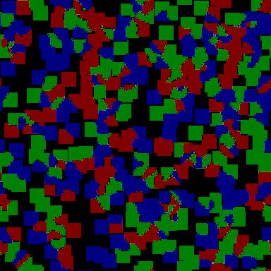
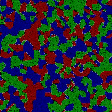
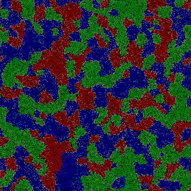
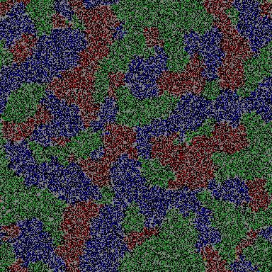
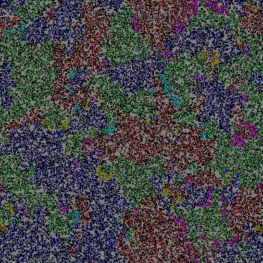

Figure 3. Time evolution of three layer system as threshold is raised. Early behaviour is similar to two layer system, but there is a range of values (approximately > 2.2 and t < 3.5) where blooms form that form leading-edges for waves.
However, at approximately 2.25 and above, narrow “blooms” of cells, active in multiple layers, but not all, start to form on the borders between regions. These blooms or fringes begin to act as leading edges that cause rapid and directed erosion into one region, with subsequent growth in another. The blooms will tend to die out after a while, with other blooms arising and taking over. The motion is quite dynamic, leading to continual movement and change in the regions.
In the three layer system, the leading-edge fringes between regions have two active layers, the layer that is expanding and the third layer which is not in either of the regions. The blooms must initially form between cells with a different layer active from the cells that they will ultimately make an edge between and then migrate. They are likely to form, for instance, near the intersection between three regions. Blooms that form between regions that share their layers and don't migrate toward another region, get eroded and disappear.
The mechanism by which the fringes act to guide erosion and growth is the following: when a cell with two layers active meets a cell with only the third layer active, the cells are deactivated. If, however, the cell touches one with all layers active, the two active layers will remain active, as these are the only shared layers. Equally, the layer which is following the leading edge will replace leading edge cells, as it is the only shared layer between it and the leading edge. The net result is movement of the edge and trailing region into the region being eroded.
As the threshold is increased, the blooms become more permanent and wider, so that by a threshold of around 3.5, regions have become basically multi-layered and the blooms have disappeared. (Figure 4.) During this transition period, as the blooms shift from being fringes to being the dominant regions, there is a period with a high level of mixing between between layers, where single layer cells are interspersed with cells with two active layers. After a time the single layer cells die out so that cells with a single layer of activation remain only on the borders, although eventually these die out, too. As the threshold is increased further, more cells appear with three active layers and the number of inactive cells continues to increase. There doesn't appear to be a period where cells with more than one active layer mix.
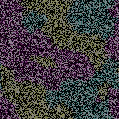
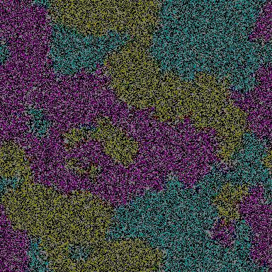
Figure 4. As threshold is raised in three layer system, regions become predominantly filled with cells with two layer activation, three layer activation and in-active cells.
When there are more than three layers, the behaviour is similar, but you get additional phase transitions at higher thresholds, where regions with multiple active layers will have fringes with even more active layers. As these transitions are approached, bubble-like, fixed regions made up of multiple active layers can form, which can last for fairly lengthy periods before being eroded. These regions generally have no inactive cells.
In these simulations, the size of regions is largely a function of active cell density in initial conditions, threshold and number of layers, with initial conditions having less effect over time if the threshold becomes high enough. Initial conditions that lead to larger, and thus more sparsely interconnected regions can lead to slightly delayed bloom formation, as there are less locations that form a nexus between multiple regions.
In general, the mechanics of this system and overall behaviour are very similar to those of reaction-diffusion systems which have been studied elsewhere, especially when the system is looked at averaged over time and space [1,12].
As all layers share the same thresholds and interact with all others in identical ways, the system as described does not seem to allow for the formation of higher-order patterns than those described, and there is no indication that it supports spontaneous multi-scale organizational patterns. Nevertheless, even though the rules of this system are acting only on nearest neighbours, the spontaneous formation of large semi-homogeneous regions, many orders of magnitude larger than individual cells, suggests that it contains at least some of the properties needed to do so. Additionally, the dynamic interactions that occur when the threshold is appropriately tuned, the leading-edge blooms or fringes, suggest the possibility for self-organization at scale. Indeed, such structures have been used to perform computation in reaction-diffusion systems, although generally not as spontaneously arising formations. Also, the ability for multiple regions to mix into inhomogeneous regions, again with appropriate threshold values, suggests that the underlying system supports structures with a significant level of local and non-local variety, which could potentially be used to control structure formation with higher levels of organization.
In the above examples, the threshold value is the dominant factor influencing the overall behaviour of the system, determining if there will be fringes, mixing, etc. However, the effect of the threshold is global. As we have seen above, varying the threshold temporally pushes the simulation into different phases. This suggests that incorporating a localized and dynamic threshold might induce the system to take on a wider range of behaviours. The range of ways in which this might be achieved is vast in principle, however, density of local activation seems like a reasonable choice, as it has some physical plausibility, and its computation requires only consideration of activation of the mask layer, which is in common between all layers. Additionally, while interesting behaviour can be observed in systems where all the layers are treated identically, having a slightly different response for each layer allows individual layers and layer combinations to act as the threshold control mechanism. Together these concepts suggest a model in which each layer maps to a specific density, and where each will only contribute to the overall activation if that exact density exists in the surrounding neighbourhood. As each layer only responds to a single density, and as there can only be a single density at a given location, only a single layer will trigger the activation. The likelihood of activation then becomes tied to the both the likely density and the number of active layers.
We use several visual analytic methods to explore the behavior of the simulation. Click on any image to open it at full resolution in a new tab.
1D Time Slices
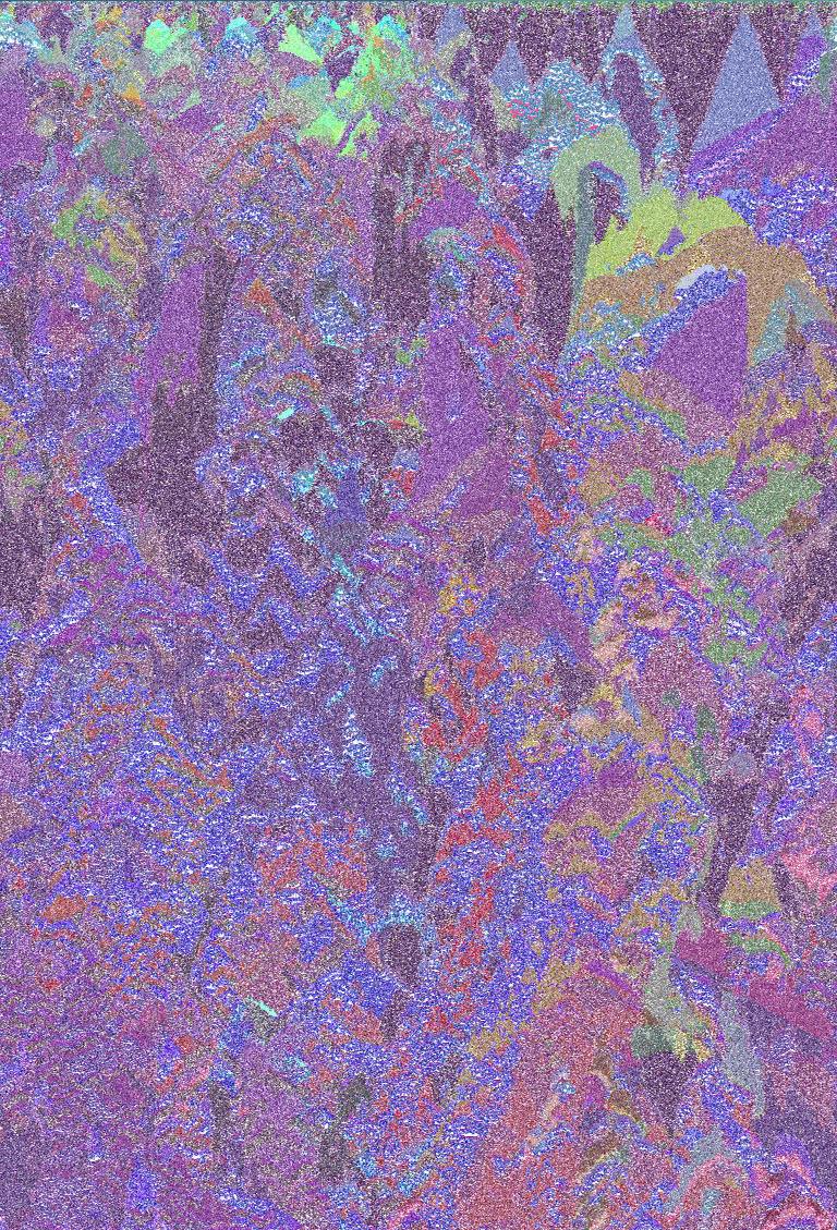
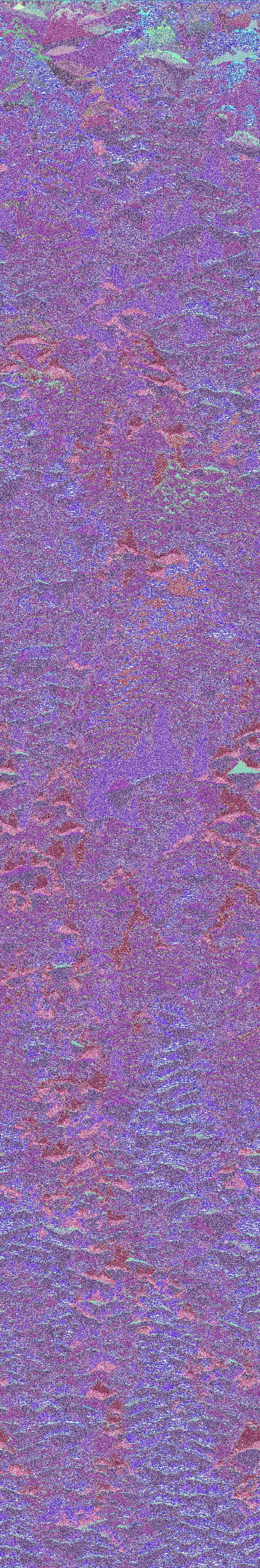
Below, we have two 1D time slices of different resolution simulations over time. The y-axis is in 10 frame intervals and the x-axis is compressed to 768 pixels.
The run on the left is a 3072x3072 size grid which ran for ~11290 frames. The run on the left is a 1536x1536 size grid which ran for ~46360 frames
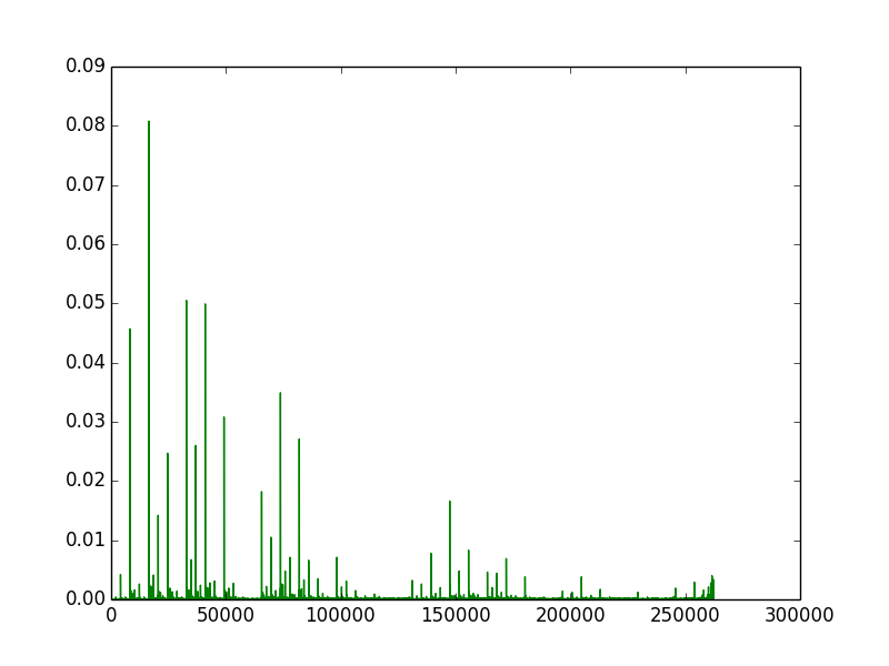
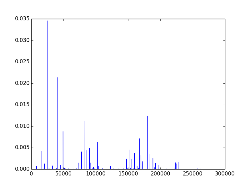
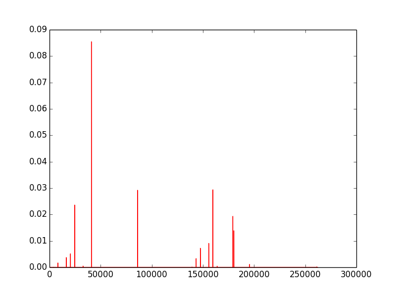
Rule Spectrum
The first image (left) is created by repeatedly running a 16x16 grid for 32 steps from random starting conditions. It is a count of all active rules, with more common rules having a larger y value. The count is based only on existence of a rule after a run, not on its frequency in the run, so very low density rules that occur in a large number of runs still get a high count. The next two images (middle and right) are produced by counting all the active rules on a given frame, and the y-axis represents the fraction of cells with that rule.
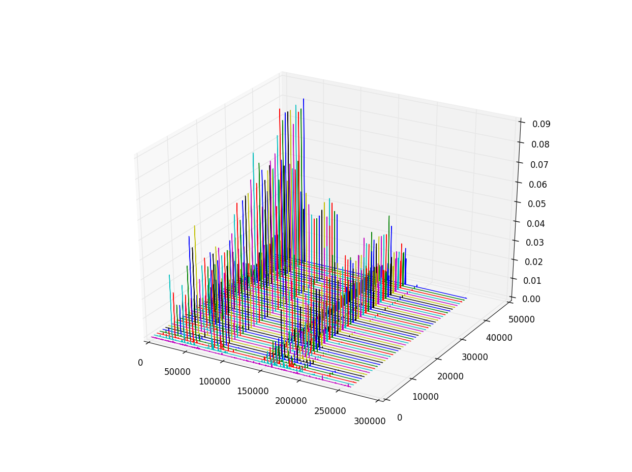
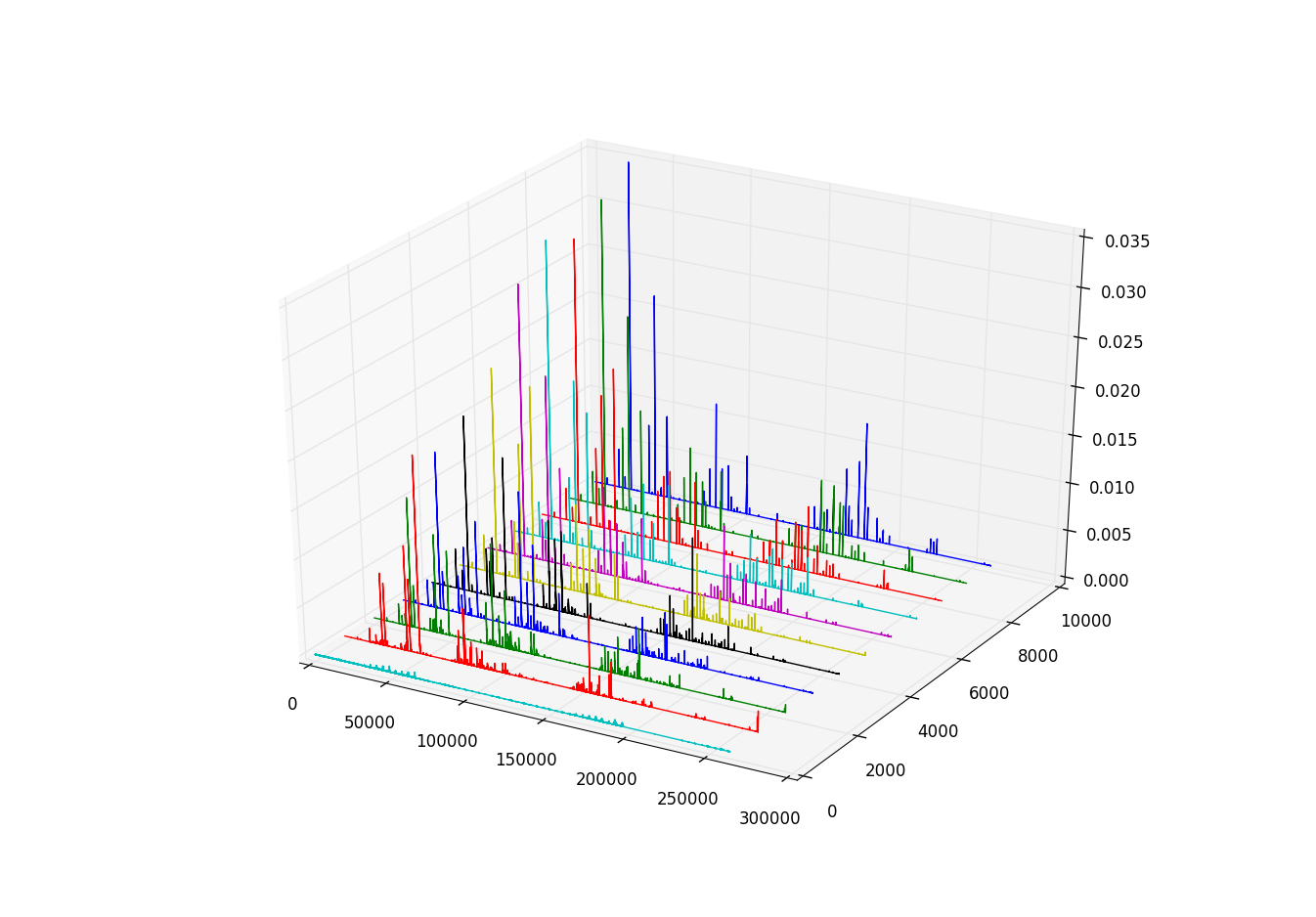
Next we look at the spectra over time as 3D plots
You can watch a video of the simulation evolving over time here and view higher resolution images here